Balancing a Pump Curve against a System Curve

Introduction

This article will demonstrate how you can balance a pump curve against a system curve to calculate liquid velocity with Excel.

First, we'll develop the equations that determine the liquid velocity in a simple pump and pipe system.  Then we'll discuss how these equations be solved using Excel's Goal Seek feature. Finally, we'll show Visual Basic code that can be used to automate Goal Seek so that any parameter change will automatically calculate the new liquid velocity.

The spreadsheet can be downloaded here, but read the rest of this article if you'd like to understand the theory.

Pump and Pipe System

Consider a centrifugal pump receiving liquid from a reservoir and forcing liquid through a pipe to a reservoir.

First consider the pump.  Its flowrate-head curve is can be described by a polynomial derived from empirical data, where a, b and c are best-fit coefficients, and Q is the volumetric flowrate

Equation 1

But the volumetric flowrate is

Equation 2

where A is the cross-sectional area of the pipe and V is the liquid velocity through the pipe.  Substituting Equation 2 into Equation 1 to eliminate Q gives

Equation 3

This equation now describes the head produced by the pump as a function of the liquid velocity through the pipe.

Now consider the pipe.  Frictional head loss through the pipe can be described by the Bernoulli equation and written as

Equation 4

We'll call Equation 4 the System Curve. f is the friction factor, given by the Haaland Equation.  

Equation 5

 where Re is the Reynolds Number.

Equation 6

The Haaland equation is only valid in turbulent flow, i.e. if the Reynolds Number is over 2500. 

For our pump and pipe system, the pump head is equal to the head loss in the pipe.  Hence

Equation 7

We can now use Excel to find the liquid velocity that satisfies Equation 7 (effectively determining the intersection between the pump curve and the system curve).

Excel Implementation

The Excel spreadsheet uses this cell coloring convention.

Step 1.  First define the parameters and calculate the cross-sectional area of the pipe.

Step 2. Now define the coefficients of the pump curve

Step 3. Set up the calculations required by Goal Seek

Step 4. Go to Data > What-If Analysis > Goal Seek.  Make the changes such that we find the liquid velocity that makes difference between pump curve and the system curve equal to zero.

You should now have the correct value of the liquid velocity.

Ensure that the Reynolds number is greater than 2500 so that our assumption of turbulent flow (and hence the use of the Haaland equation) is verified.

Visual Basic Macro to Automate Goal Seek

If you're really keen, you can use Visual Basic to automate Goal Seek.

Private Sub Worksheet_Change(ByVal Target As Range)

Dim bSuccess As Boolean
    On Error Resume Next
    bSuccess = Range("C23").GoalSeek(0, Range("c18"))
    On Error GoTo 0
    If Not bSuccess Then
        MsgBox "Goal Seek Failed"
    End If
End Sub

Whenever any value in the worksheet is changed, the Worksheet_Change() event is initiated .  The VB code then asks GoalSeek() to find the liquid velocity ("C18") that makes the difference between the pump and system curve ("C23") equal to zero.

Download Excel Spreadsheet to Balance a Pump Curve Against a System Curve

The Three Reservoir Problem

Introduction
This article discusses how you can solve the Three Reservoir Problem with Excel. First, we develop the governing equations by applying Bernoulli's Equation and the Continuity Equation. We then explore how these equations can be solved in Excel.

If you just want the tutorial spreadsheet, click here, but I encourage you to read the rest of the article so you understand how the spreadsheet was developed.  Read on for the Three Reservoir Problem solution.

Theory

Three reservoirs at different elevations are connected by a pipe network.  The common junction of the piping network is subject to an external demand Qj of 0.01 m3/s.  We will develop the theory required to calculate the flowrates in each pipe (Q1, Q2 and Q3), the head at the junction (Hj) and determine whether liquid is flowing into or out of each reservoir

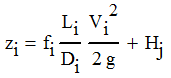
Assuming that the liquid level in each reservoir is constant and the surface is open to atmosphere, the Bernoulli Equation for Reservoir i (where i=1, 2 and 3) is

Equation 1

where zi is the elevation, fi is the friction factor, Li and Di are the length and diameter of the pipe connecting the reservoir to the junction, Vi is the liquid velocity and g is the gravitational constant.

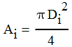
But the volumetric flowrate Qi and the cross sectional area Ai of the pipe are

Equation 2

Equation 3

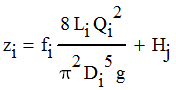
Substituting Equations 2 and 3 into Equation 1 to eliminate Vi gives

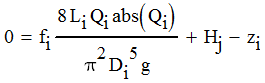
Equation 4

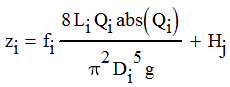
To determine whether liquid is flowing into or out of a reservoir, we need to preserve the sign on the Qi^2 term by writing Equation 4 thus

Equation 5

If Qi is positive, liquid is flowing out of the reservoir, and if Qi is negative, liquid is flowing into the reservoir.

We only need a few more relationships to completely specify the system.  The friction factor fi is given by the Haaland approximation to the Colebrook-White Equation,

where Rei is the Reynolds Number,

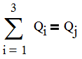
Additionally, the sum of the flowrates from each reservoir is equal to the external demand

Excel Implementation
Moving all terms in Equation 5 to the right-hand side gives

Equation 6

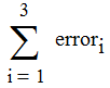
However, if we don't know the exact values of the flowrates in each pipeline (Qi) or the head at the junction (Hj) then we can define an error for each pipe.

Equation 7

We'll use Excel's Solver add-in to find the values of Q1, Q2, Q3 and Hj that minimize the total error...

Equation 8

...while keeping the total flowrate at the junction equal to the external demand.

Equation 9

Step1. Specify fixed parameters (such as densities, viscosities, reservoir heights, pipe diameters and roughnesses etc)

Step 2. Set initial guess values for the flowrates in each pipe

  

Step 3. Specify calculated values

Step 4. Specify an initial guess value for the head at the junction, and the sum of all flowrates in each pipe (as given by Equation 9).  The External Demand will act as the constraint for Excel's Solver

Step 5.  Specify the errors for each pipeline (as given by Equation 7), and the total error (as given by Equation 8). 

We can now use Excel's Solver Add-in to find the flowrates (Q1, Q2 and Q3) and head at the junction (Hj) that minimize the total error (as set in Step 5) subject to the flowrate constraint (as set in Step 4).

Step 6.  Initiate Excel's Solver menu (if you haven't already, you'll need to load it in the File > Options > Add-ins menu)

Step 7. Make the appropriate changes in the Solver window such that you minimise the total error by varying the flowrates and the junction head while maintaining the external demand at a set value (for this example, I've set the external demand to 0.01 m3/s).  Additionally, set the solving method to GRG Nonlinear.

Step 8.  Click Solve.  After dismissing the following window, you'll find that the flowrates in each pipeline, and the junction head have changed.  Bear in mind that positive flowrates indicate flow out of a reservoir, while negative flowrates indicate liquid flow into a reservoir.

Step 9. We're not finished yet! Check that the Total Error specified in Step 5 is a very small number, and the External Demand (in Step 5) is equal to the value specified in Step 7.

Download Excel spreadsheet to solve The Three Reservoir Problem