Modelling Reaction Kinetics in Excel

This spreadsheet demonstrates how you can model reaction kinetics in Excel with the solution of differential equations.

Consider this reaction scheme

where A and B are reactants, X and Y are catalysts, and k₁ and k₂ are rate constants.

The following coupled differential equations can be derived from the stoichiometry of the chemical reaction scheme.

where a(t), b(t), x(t) and y(t) are the concentrations of A, B, X and Y at time t. This is an initial value problem, where the concentrations x(t), y(t), a(t) and b(t) must be specified at time t = 0.

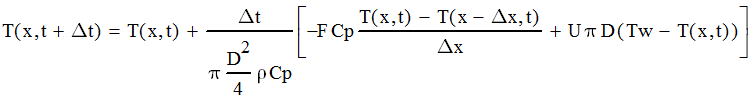
These differential equations can be easily solved in Excel using a simple forward-stepping finite difference scheme. The differential equations are discretized as follows

where Δt is the chosen time step. As long as Δt is sufficiently small, the solution will be accurate.

This is an initial value problem, where a(0), b(0), x(0) and y(0) need to be specified. The following picture illustrates the implementation in Excel.

These are typical results for the concentration profile of the reactants.

The concentrations of the catalysts X and Y return to the values specified at the start of the simulation, as the reaction proceeds.

The principles illustrated here can be used to solve any other initial value differential equations arising from reaction kinetics in Excel.

Download Excel Spreadsheet to Model Reaction Kinetics (Solution of Initial Value DEs via Finite Difference)

Dynamic Liquid Flow Between Coupled Tanks

This Excel spreadsheet models the transient flow of liquid between two tanks connected by a pipe.  Because of the momentum of the liquid, the height of liquid in each tank oscillates to an equilibrium.  Flow is opposed by pipe friction, and eventually the liquid level in each tank stabilises.

The dynamics are defined by the following differential equations, which are derived from a mass balance and momentum balance (ref: "Chemical Engineering Dynamics: An Introduction to Modelling and Computer Simulation" by John Ingham et al).

• H₁(t) and H₂(t) are the height of liquid in each tank
• A₁ and A₂ are the cross-sectional area of each tank
• Q is the flowrate in the pipe (m³ s^-1
• ρ is the liquid density (kg m^-3)
• μ is the liquid viscosity (Pa s)
• g is the gravitational constant (9.81 m s^-2)
• L is the length of the pipe (m)
• D is the pipe diameter (m)
• e is the pipe roughness (m)
• Re is the Reynolds number
• f is the friction factor (for Re < 2000, f is given by 64/Re, while for Re ≥ 2000 f is given by the Haaland equation)

The differential equations are solved in Excel with a simple finite difference Euler scheme, as described by these equations

The spreadsheet is straightforward to use.  Simply enter your parameters.

The spreadsheet will then calculate the flowrate in the pipe, and the change in liquid height in each tank over time. Note that the first row of the results (at t=0) contain the initial conditions.  These can be changed.

The spreadsheet also plots the liquid height in each tank over time.  As you can see, the level of each tank oscillates over time, with the flow being damped by friction.  Eventually,  the height of liquid in each tank reaches an equilibrium level.

Download Excel Spreadsheet to Model Dynamic Liquid Flow Between Two Tanks

Dynamic Model of a Cross-Flow Heat Exchanger

Introduction
This article will develop a dynamic model of a cross-flow heat exchanger from first principles, and then discretize the governing partial differential equation with finite difference approximations.  It will then demonstrate how this equation can be implemented in Excel (or indeed any other math tool)

If you just want the Excel implementation, then click here, but I encourage you to read the rest of the article so you understand how the spreadsheet is implemented.

First Principles Modeling
Consider liquid flowing (at mass flowrate F) through a length Δx of pipe (diameter D), subject to cooling by cross-flow air (at temperature Ta and heat transfer coefficient U)

A heat balance over time Δt gives the following.

 

Dividing by Δx and Δt and simplifying gives

As Δx and Δt tend to zero, we get the following parabolic partial differential equation

Equation 1

Finite Difference Approximation

A forward difference approximation for the first of temperature with respect to time is

Equation 2

A backward difference approximation for the first of temperature with respect to space is

Equation 4

Substituting Equation 2 and 3 into Equation 1, and rearranging gives

Equation 4

We only need to know the temperature of the bar at time t (on the RHS of Equation 4) to calculate the temperature at time t + Δt (on the LHS of Equation 4).

Implementating in Excel

This is how Equation 4 will be implemented in Excel

We will now discuss the individual steps in detail.

Step 1  - Specify your parameters, including your chosen time and space step.  I've named the cells in Column C with the names in Column E.  I'll use named values when entering Equation 4.

Step 2 - Create a column and row containing your space and time steps

Step 3 - Fill in your initial conditions at time t = 0 (this will be the inlet liquid temperature as specified in the parameters).

Step 4 - Insert your boundary conditions at distance x = 0 (this will be the inlet liquid temperature - the same as the initial condition).

Step 5 - Implement Equation 4 into the first empty cell (at t = Δt and x = Δx)

Step 5 - Copy this formula to all other times and positions.  For my implementation, I go up to t = 1 and x = 0.4.

The techniques I've demonstrated above can be applied to many other challenges in science, engineering and math.  If you have any requests, then let me know.

Download the Excel 97 spreadsheet that models a Cross-Flow Heat Exchanger

Solving the 1D Heat Equation Using Finite Differences

Introduction
The Heat Equation describes how temperature changes through a heated or cooled medium over time and space.  In one dimension, the heat equation is

1D Heat Equation

This post explores how you can transform the 1D Heat Equation into a format you can implement in Excel using finite difference approximations, together with an example spreadsheet. If you just want the spreadsheet, click here, but please read the rest of this post so you understand how the spreadsheet is implemented.

We will model a long bar of length 1 at an initial uniform temperature of 100 C, with one end kept at 100 C.

 

Finite Difference Approximations
The central and forward difference approximations for the 1st derivative wrt time and the 2nd derivative wrt space are

Forward and central difference approximations

Substituting these relationships into the heat equation and rearranging gives an equation that describes the temperature u at position x along the bar and time t+Δt. 

Equation 1

Equation 1 is in a form that can be implemented in Excel.  Note that we only need to know the temperature of the bar at time t to know the state at time t+dt, as illustrated below.

Boundary Conditions
Now lets define the initial and boundary conditions. The left-hand side (i.e. x=0) of the bar is kept at a fixed temperature of 100 C , while the initial temperature is 0 C.

We also need a boundary condition on the right hand side of the bar at x=1.  The rate of change of temperature with respect to distance on right hand side of the bar is 0.

A central difference approximation to this boundary condition is

Rearranging this gives

Equation 2

Now, Equation 1 on the right-hand boundary (at x=1) can be rewritten

Equation 3

 Substituting Equation 2 into Equation 3 so that we eliminate u(1+Δx, t) we get

Equation 4

Equation 4 describes the boundary condition on the right-hand side of the bar in a form that can implemented in Excel

Excel Implementation
To summarize, now we have

• Equation 1 - the finite difference approximation to the Heat Equation
• Equation 4 - the finite difference approximation to the right-hand boundary condition
• The boundary condition on the left u(1,t) = 100 C
• The initial temperature of the bar u(x,0) = 0 C

This is all we need to solve the Heat Equation in Excel.  This screengrab represents how the system can be implemented, and is color coded according to the legend below.

Rows represents the distance along the bar, with time increasing as you go down.

If you want the Mathcad implementation, then click here.

Download Excel 97 spreadsheet for solving 1D Heat Equation