Velocity Profile in a Circular Pipe

This Excel spreadsheet calculates and plots the velocity profile of a power-law fluid in a circular pipe. The spreadsheet is valid for Newtonian, pseudoplastic and dilatant fluids.

The velocity profile of a Power-law fluid is given by this equation.

where

• r is the radial position i.e. distance from the center line (m)
• R is the pipe radius (m)
• u(r) is the axial velocity (m s^-1)
• dp/dz is the axial pressure gradient (Pa m^-1)
• K is the flow consistency index (Pa sⁿ)
• n is the flow behavior index

The equation above is only valid for developed steady-state laminar flow in a circular pipe. The entrance length (that is, the pipe length needed to develop a steady-state velocity profile) for laminar flow is given by this correlation.

The value of n determines the relationship between the axial velocity and radial distance. If

• n = 1, the fluid is Newtonian
• n < 1, the fluid is pseudoplastic
• n > 1, the fluid is dilatant

The chart below gives the velocity profile for different values of n (with all other parameters constant).

The spreadsheet is simple to use. Simply enter the parameters

Excel will then plot the velocity profile from the centerline to the surface of the pipe. As expected, the velocity profile is symmetrical.

The transient velocity profile in laminar flow is more difficult to calculate; this requires the numerical solution of a partial differential equation via a finite difference scheme. This will be the subject of another spreadsheet.

Download Spreadsheet to Calculate the Velocity Profile in a Circular Pipe

Calculate Gas Viscosity with Sutherland's Law

This Excel spreadsheet calculates the viscosity of gasses with Sutherland's Law. The spreadsheet contains constants suitable for air, but can be used for other gases.

William Sutherland was an Australian scientist who studied the temperature-dependence of ideal gases. In 1893, he developed an empirical-theoretical relationship between the temperature and viscosity of an ideal gas.

Essentially, the method uses a known reference viscosity and temperature to find another viscosity at a specified temperature.

Sutherland's formula is

 where

• μ is the dynamic viscosity (Pa s or kg m^-1 s^-1)
• T is the temperature (K)
• μ_ref is a reference viscosity (Pa s or kg m^-1 s^-1)
• T_ref is a reference temperature (K)
• S is the Sutherland Constant for the gas (K)

The Sutherland Constant is characteristic for the gas. For example, 

• air at 323 K has a viscosity of 1.716 x 10^-5 Pa s, with a Sutherland Constant of 110 K
• helium at 273K has a viscosity of 1.9 x 10^-5 Pa s, with a Sutherland Constant of 79.4 K

The spreadsheet also

• finds the density of the gas with the Ideal Gas Law
• calculates the kinematic viscosity by dividing the dynamic viscosity by the gas density

The Ideal Gas Law is given by this formula

where

• R is the Universal Gas Constant (8314.4 J kmol^-1 K^-1)
• M is the molecular weight of the gas (kg kmol^-1)
• P is the pressure (Pa)
• ρ is the density (kg m^-3)

The molecular weight of air, for example, is 28.96 kg kmol^-1.

Sutherland's Law is accurate for moderate temperatures and pressures, and also describes the viscosity-temperature relationship of gasses at hypersonic speeds.

Download Excel Spreadsheet to Calculate Gas Viscosity with Sutherland's Law

Historical Crude Oil Prices

These two Excel spreadsheets automatically download historical crude oil prices straight into Excel. Both tools are fully automated; the most you do is supply dates and click a button.

Some VBA then downloads the data from a 3rd party website, straight into Excel. After the data is in Excel, you can do whatever you want - visualize price historical, perform economic analysis, correlate oil prices against the cost of other raw materials, and more.

The first spreadsheet downloads Brent oil price data, while the second downloads historical prices for West Texas Intermediate .

The price of crude oil effects the price of everything we use or consume, including food, fertilizers, gasoline and household electronics. It also influences the price of other industrial chemicals, and accordingly is a major economic factor in the chemical and process industries.

Both spreadsheets are available at my other site, InvestExcel

Download Excel Spreadsheet to Automatically Retrieve Historical Brent Oil Price Data

Download Excel Spreadsheet to Automatically Retrieve Historical WTI Oil Price Data

Heat Loss From An Insulated Pipe

This Excel spreadsheet models heat loss from an insulated pipe. This is a very common system in the process industries - insulated pipes are everywhere, and engineers need a sound grasp of heat transfer principles to model their effects. Although the model in the spreadsheet is simplified to aid understanding, complexity can be easily added.

Liquid flows through the pipe, with heat exchanged with the insulation. Heat is lost from the insulation to the environment via convection (no radiation losses are considered). The thermal effects of the pipe wall are ignored (although this can be easily implemented).

These equations are used in the spreadsheet to define the heat transfer process.

• q is the heat flowrate through the pipe and insulation (W m^-1)
• T_s is the temperature at the surface of the insulation (K)
• T_a is the ambient air temperature (K)
• T_f is the fluid temperature inside the pipe (K)
• D_O is the pipe diameter (m)
• D_S is the outside diameter of the insulated pipe (i.e. the pipe diameter plus two times the insulation thickness) (m)
• k is the insulation thermal conductivity (W m^-1 K^-1)
• ΔT is the temperature difference between the insulation surface and ambient air T_s-T_a (K)
• h_s is the insulation-to-air heat surface heat transfer coefficient (W m² K^-1)

The equation for the surface heat transfer h_s coefficient is a correlation; any other valid relationship can be substituted.

The equations are implicit - the heat transfer coefficient is a function of the surface temperature T_s, but the surface temperature is a function of the heat transfer coefficient. 

Hence the equations need to be solved iteratively with Goal Seek in Excel. Simply 

• break the loop by estimating a value of T_s, 
• use this to calculate all other properties (including the heat transfer rate)
• use the heat transfer rate to backcalculate T_s
• use Goal Seek to make the two values of T_s equal by varying the estimated value of T_s (or any other parameter

You can easily modify the heat transfer equations to include more complex effects, such as effect of fouling on the pipe surface, multiple layers of different insulation, radiative losses, thick large pipe walls (which act as a heat sink) etc.

Download Excel Spreadsheet to Model Heat Loss from Insulated Pipe

Calculate d-Exponent to Predict Pore Pressure Trends

This Excel spreadsheet calculates the d-exponent, a parameter used by drilling engineers to investigate ppore pressure trends when drilling into over-pressurized zones.

Normally, formation density increases with the drilling depth. But if the formation contains sand below the surface, then the drilling rate may increases with drilling depth. The d-exponent is used in several calculations to investigate these effects.

Jorden and Shirley (1966) suggested the d-exponent method, basing it on the Bingham equation. A later adjustment to the equation by Rehm and Mcledon (1971) included the effect of mud weight

The modified equation to calculate the d-exponent is

where

• c is the shale compactibility coefficient
• ρ_n is the mud weight equivalent (lb gal^-1)
• ρ_m is the mud weight used (lb gal^-1)
• D is drill bit diameter (in)
• W is the weight on the bit (x 1000 lb)
• R is the penetration rate (rpm)
• N is the rotary speed.

The d-exponent is often used in Eaton's equation

where

• P is the formation pore pressure (psi)
• P_ob is the overburden pressure (ft)
• Z is the vertical depth (ft)
• d is the d exponent
• d_n is the normal compaction trend of the d exponent
• P_p is the formation pore pressure (psi)
• P_p/Z is the normal pore pressure gradient (psi ft^-1)

Download Excel Spreadsheet to Calculate D Exponent

Modelling Reaction Kinetics in Excel

This spreadsheet demonstrates how you can model reaction kinetics in Excel with the solution of differential equations.

Consider this reaction scheme

where A and B are reactants, X and Y are catalysts, and k₁ and k₂ are rate constants.

The following coupled differential equations can be derived from the stoichiometry of the chemical reaction scheme.

where a(t), b(t), x(t) and y(t) are the concentrations of A, B, X and Y at time t. This is an initial value problem, where the concentrations x(t), y(t), a(t) and b(t) must be specified at time t = 0.

These differential equations can be easily solved in Excel using a simple forward-stepping finite difference scheme. The differential equations are discretized as follows

where Δt is the chosen time step. As long as Δt is sufficiently small, the solution will be accurate.

This is an initial value problem, where a(0), b(0), x(0) and y(0) need to be specified. The following picture illustrates the implementation in Excel.

These are typical results for the concentration profile of the reactants.

The concentrations of the catalysts X and Y return to the values specified at the start of the simulation, as the reaction proceeds.

The principles illustrated here can be used to solve any other initial value differential equations arising from reaction kinetics in Excel.

Download Excel Spreadsheet to Model Reaction Kinetics (Solution of Initial Value DEs via Finite Difference)

Souders-Brown Equation Calculator

This Excel spreadsheet calculates the maximum allowable vapor velocity in a vapor-liquid separator with the Souders-Brown equation. The Souders-Brown equation is commonly used to size separators, scrubbers and knock-out drums.

The operating vapor velocity is specified to minimize the entrainment of liquid drops in the exiting vapor.

A wire mesh or de-entrainment pad is commonly used to force the separation of very small drops that cannot be removed by gravity alone. These coalesce the smaller droplets into larger ones fall due to the force of gravity.

Vapor-liquid separators are commonly used in the oil & gas, petrochemical industries, paper mills

The Souders-Brown equation was derived from a force balance on a droplet suspended in a gas flowing upwards. It was originally derived to size fractionating columns.

This is the equation.

• ρ_L is the liquid density (kg m^-3)
• ρ_L is the gas density (kg m^-3)
• K is the vapor or gas load factor (m s^-1)
• V is the maximum allowable vapor velocity (m s^-1)

K has a value of 0.107 m s^-1 for a separator with a mesh pad. However, the right value of K is largely dependent on the operating conditions and physical properties of the system. The GPSA Engineering Data Handbook tabulates values of K for various operating conditions.

Once you have the maximum allowable vapor velocity, you can then calculate the drum diameter by dividing the vapor flowrate by the allowable vapor velocity.

Download Excel Spreadsheet for the Souders-Brown Equation

Inflow Performance Relationship of Vertical & Slanted Solution Gas-Drive Wells

This Excel spreadsheet calculates the Inflow Performance Relationship, or IPR, for vertical and slanted solution-gas drive wells.

The IPR of a well determines the relationship between its flowing bottom pressure, and the well production rate (or deliverability). IPR also helps engineers investigate the economics of a well, and is critical in optimizing the well, artificial lift design and determining the nature of the surface equipment.

For single-phase fluids, the IPR relationship is linear. However, when two-phase liquid and gas below its bubble-point pressure are produced, the relationship is non-linear.

Several researchers have studied this process, most notably Vogal (1968) and Cheng (1990). Cheng's semi-empirical correlation is applied to slanted wells, while Vogal's work applies to vertical wells.

Vogel and Cheng's equations are

where

• q₀ is the flow rate in bbl/day
• q_0,max is the oil flow rate at a flowing bottom hole pressure of 0 in bbl/day
• p_wf is the flowing bottom hole pressure in psi
• p_r is the reservoir pressure in psi
• a₀, a₁ and a₂ are empirical parameters that vary with the slant angle. In the spreadsheet these parameters are listed again several values of the slant angle. Intermediate values are linearly interpolated.

Download Excel Spreadsheet to Calculate Inflow Performance Relationship for Solution-Drive Gas Well

Ergun Equation Calculator

This Excel spreadsheet helps you calculate the pressure drop through packed and fluidizeds bed with the Ergun equation.

Fluidized beds are a commonly unit operation in the process industries. Their nature makes them particularly suitable venues for gas-solid catalyzed reaction, often in the petroleum industry to produce gasoline and other chenicals. They have also found use in the polymer industry, and bioreactors (in the form of liquid fluidized beds)

In 1952, Sabri Ergun derived the following equation to predict the pressure drop in packed beds.

• ΔP is the pressure drop
• L is the height of the bed
• D_p is the particle diameter
• ε is the porosity of the bed
• μ is the gas viscosity
• V₀ is the superficial velocity (the volumetric gas flowrate divided by the cross-sectional area of the bed)
• ρ_g is the gas density

The pressure drop required for minimum fluidization is given by

• ρ_p is the particle density
• ε_M is the porosity of the bed at minimum fluidization

By comparing the pressure drop given by the Ergun equation to the pressure drop for minimum fluidization, you can calculate the superficial velocity necessary for fluidization. At this point, bubbles of gas form and rise through the bed. This increases the effective volume of the bed.

Download Excel Spreadsheet to Calculate Ergun Equation

Liquid Volume in Partially Filled Horizontal Tanks

This Excel spreadsheet helps you calculate the liquid volume in partially filled horizontal tanks.

Tanks are often used in storing chemicals. Often, only the liquid height from a level indicator is known. This means you need a method of calculating the liquid volume based on the liquid height and the tank dimensions.

The tank ends can be

• flat (so the tank is just a horizontal cylinder)#
• dished (ASME F&D, or Flanged & Dished)
• 2:1 elliptical 
• hemispherical

The liquid volumes in a horizontal cylinder, and ASME F&D, 2:1 elliptical and hemispherical ends are given by these equations.

where

• D is the diameter of the cylinder and the heads
• L is the length of the cylindrical shell
• h is the height of liquid in the tank

The diagram at the top illustrates the notation.

Hence the total volume of liquid in the tank is simply the liquid volume in the cylinder plus 2 times the liquid volume in the heads.

The dimensions can be specified in any length unit. The unit of the volumes will simply be the length unit cubed.

This spreadsheet can be easily modified to created a Dip chart (i.e. a chart giving the liquid volume as a function of liquid height).

Download Excel Spreadsheet to Calculate Liquid Volume in Partially Filled Tanks

Fetkovich Decline Curve Analysis

This Excel spreadsheet plots Fetkovich decline curves for gas wells. Decline curve analysis is an empirical procedure that predicts the decline in production rates of gas and oil wells. 

Fetkovich (1968) improved on earlier work by Arps in predicting the declining production rate of oil and gas wells. He suggested that experimental production rate data could be overlaid on a graph and matched to a series of type curves. The production rate is then extrapolated into the future with the assistance of the curves.

The Excel spreadsheet reproduces the plot given in Figure 8 of the following reference.

Fetkovich, M.J., "Decline Curve Analysis Using Type Curves", Journal of Petroleum Technology (June 1980) 1065-77.

The decline curve rate-time equations are given below.

where

• n is a factor that governs the shape of the back pressure curve
• q_Dd is the decline curve dimensionless production rate
• t_Dd is the decline curve dimensionless time

Download Excel Spreadsheet to Plot Fetkovich Decline Curves for Gas Reservoirs

Water Breakthrough Time in a Vertical Oil Well

Consider an oil reservoir with an underlying water zone. An oil well that is producing from this reservoir will experience the phenomenon of water breakthrough if the well produces above its critical rate. Since economic considerations often demand high flowrates, this can be a real risk.

This Excel spreadsheet uses the Sobocinski-Cornelius method to calculate the water breakthrough time.  This method was published in 1965, and was derivied from laboratory tests. It uses these equations.

where

• B_o is the oil formation volume factor
• μ_o is the oil viscosity (cp)
• μ_w is the water viscosity (cp)
• φ is the porosity
• h is the oil column thickness (ft)
• h_p is the perforated interval (ft)
• Q_o is the oil production rate (STB day^-1)
• α is 0.5 if M <=1, or 0.6 otherwise
• M is the water-oil mobility ratio
• t_BT is the time to breakthrough
• t_D is the dimensionless time (Sobocinski-Cornelius method)
• Z is the dimensionless cone height
• ρ_w is the water viscosity (lb ft^-3)
• ρ_o is the oil density (lb ft^-3)

Download Excel Spreadsheet to Calculate Water Breakthrough Time with Sobocinski-Cornelius method

Binary Distillation with McCabe-Thiele Method

This Excel spreadsheet uses the McCabe-Thiele method to calculate the number of theoretical stages needed for binary distillation.

Binary distillation is a common unit operation that separates two liquids (with one being more volatile, or "lighter"). The concepts are encountered in many branches of chemical and petroleum engineering.

Simply enter your parameters at the top of the spreadsheet, including the

• feed flowrate,
• mole fraction of the light component (or more volatile component) in the feed,
• mole fraction of light component in the top product,
• mole fraction of light component in the bottom product,
• reflux ratio,
• relative volatility of the light component
• and the q-line value.

The spreadsheet will automatically calculate flowrates throughout the column, the number of theoretical plates, the feed plate position, the minimum reflux ratio (from the Underwood equation), and the minimum number of theoretical plates (from the Fenske equation)

The spreadsheet also automatically draw the traditional McCabe-Thiele plot. This is a classic Chemical Engineering diagram and shows the number of theoretical stages, the position and slope of the q-line, and the relative volatility curve, and the purity of the top and bottom products.

Download Excel Spreadsheet for Binary Distillation with McCabe-Thiele Method

Flow Regime Map for Two-Phase Flow

This Excel spreadsheet plots a flow regime map for the two-phase flow of liquid and gas in horizontal and vertical pipes.

Determining flow regime is important when calculating pressure drops and pumping requirements in the oil & gas industry, and chemical production. Additionally, some flow regimes are undesirable (such as slug flow, which can damage pipes through excessive vibration). Engineers will change pipe diameters and other process parameters so the flow regime is more favorable.

In the spreadsheet, simply enter the liquid and gas flowrates.

The spreadsheet will then plot the location of the flow on a flow regime map for horizontal and vertical pipes. The horizontal and vertical axes are the Gas Froude Number and Liquid Froude Number.

The spreadsheet uses the flow regime maps digitized from Shell DEP 31.22.05.11 (the "DEP" is short for Design and Engineering Practice")

Many flow regime maps have been developed by different researchers. For example, 

• Mandhane et al (1974) published a map for two-phase horizontal flow
• Hewitt and Roberts (1969) published a map for two-phase vertical flow
• Taitel and Dukel (1976) published a map for two-phase horizontal flow

There are, however, inconsistencies in the definition of flow regimes in these different maps. For example, some maps give different flow regimes at the same conditions.

The horizontal and vertical maps given in Shell DEP 31.22.05.11 were developed by a single source, and have a consistent definition of flow regimes.  Therefore, engineers can compare potential flow regimes in horizontal and vertical pipes.

Download Excel Spreadsheet to Calculate and Plot Flow Regime in Two-Phase Flow in Horizontal & Vertical Flow

Natural Gas Viscosity with Carr, Kobayashi, and Burrows Correlation

This Excel spreadsheet uses the Carr, Kobayashi, and Burrows correlation to calculate the viscosity of natural gas. The correlation is valid for sweet and sour gas.

The Carr, Kobayashi, and Burrows correlation was published in 1954. It is valid between temperatures of 32 F to 400 F, reduced pressures below 20, and CO₂, N₂ and H₂S concentrations below 15%.

The correlation was originally presented in graphs. However, this spreadsheet contains polynomial curve fits to the original graphs given by Dempsey (1965).

This spreadsheet also corrects calculates the viscosity (Standing & Katz, 1977) and pseudo-critical temperature/pressure of natural gas, but corrects for the presence of CO₂, N₂ and H₂S.

A spreadsheet to calculate the viscosity of natural gas based on the Lee, Gonzalez and Eakin correlation is also available; this method, however, is only valid for sweet natural gas.

Download Excel Spreadsheet to Calculate Natural Gas Viscosity using Carr, Kobayashi and Burrows

Water Hammer in Excel

This Excel spreadsheet will calculate the maximum pressure surge when the valve at the end of a pipeline is closed.

When flow is suddenly stopped, flow inertia causes a pressure surge at the valve, with a shockwave propagating through the pipeline.  This  is also known as Water Hammer and can cause considerable damage.  Engineers need to know the maximum pressure surge to correctly design the pipe, valve andother fittings.

Water hammer is a common phenomenon. For example, the audible creaking when taps are shut off in kitchens or bathrooms results from the Water Hammer effect

These are the equations implemented in the spreadsheet.

where

• K is the bulk modulus of the liquid (Pa)
• ρ is the liquid density (kg m ^-3)
• D is the pipe diameter (m)
• t is the pipe wall thickness (m)
• E is the Young's Modulus of the pipe (Pa)
• c is the speed of sound in the pipe (m s^-1)
• Δv is the velocity of the liquid before the valve is shut  (m s^-1)
• ΔP is the maximum pressure (at the valve) generated by the valve closure(Pa)

Δv can be easily calculated by the Darcy-Weisbach equation. ΔP is also known as the Joukowsky Pressure.

These equations do not predict the pressure surge arising from column separation (which may be higher than the Joukowsky Pressure). Column separation references the breaking of liquid columns in filled pipes.

Download Excel Spreadsheet for Water Hammer

Dynamic Liquid Flow Between Coupled Tanks

This Excel spreadsheet models the transient flow of liquid between two tanks connected by a pipe.  Because of the momentum of the liquid, the height of liquid in each tank oscillates to an equilibrium.  Flow is opposed by pipe friction, and eventually the liquid level in each tank stabilises.

The dynamics are defined by the following differential equations, which are derived from a mass balance and momentum balance (ref: "Chemical Engineering Dynamics: An Introduction to Modelling and Computer Simulation" by John Ingham et al).

• H₁(t) and H₂(t) are the height of liquid in each tank
• A₁ and A₂ are the cross-sectional area of each tank
• Q is the flowrate in the pipe (m³ s^-1
• ρ is the liquid density (kg m^-3)
• μ is the liquid viscosity (Pa s)
• g is the gravitational constant (9.81 m s^-2)
• L is the length of the pipe (m)
• D is the pipe diameter (m)
• e is the pipe roughness (m)
• Re is the Reynolds number
• f is the friction factor (for Re < 2000, f is given by 64/Re, while for Re ≥ 2000 f is given by the Haaland equation)

The differential equations are solved in Excel with a simple finite difference Euler scheme, as described by these equations

The spreadsheet is straightforward to use.  Simply enter your parameters.

The spreadsheet will then calculate the flowrate in the pipe, and the change in liquid height in each tank over time. Note that the first row of the results (at t=0) contain the initial conditions.  These can be changed.

The spreadsheet also plots the liquid height in each tank over time.  As you can see, the level of each tank oscillates over time, with the flow being damped by friction.  Eventually,  the height of liquid in each tank reaches an equilibrium level.

Download Excel Spreadsheet to Model Dynamic Liquid Flow Between Two Tanks

Darcy-Weisbach Equation for Liquid Velocity in a Pipe

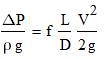
This Excel spreadsheet uses the Darcy-Weisbach equation to calculate liquid velocity in a pipe.  The Darcy-Weisbach equation describes the relationship between the pressure loss and liquid velocity in a pipe.

This is the equation employed in the spreadsheet.

• ΔP is the pressure loss in the pipe (Pa)
• ρ is the liquid density (kg m^-3)
• μ is the liquid viscosity (Pa s)
• g is the gravitational constant (9.81 m s^-2)
• L is the length of the pipe (m)
• D is the pipe diameter (m)
• V is the liquid velocity (m s^-1)
• f is the Darcy Fanning friction factor

For laminar flow (Re<2000), the friction factor f is 64/Re (where Re is the Reynolds Number). Ror turbulent flow the friction factor is given by the Haaland equation (although the Colebrook equation can be used instead).


The calculation is iterative, and requires the use of Excel's Goal Seek. However, this is automated in the spreadsheet so you only have to click a button and some VBA initiates Goal Seek for you.

The Darcy-Weisbach equation should only be used for steady-state incompressible flow. It can also be used for open-channel flows by replacing the diameter with the 4 R, where R is the hydraulic diameter.  The hydraulic diameter is simply the cross-sectional area divided by the wetted perimeter.

Download Excel Spreadsheet to use Darcy-Weisbach Equation to Calculate Liquid Velocity