Darcy-Weisbach Equation for Liquid Velocity in a Pipe

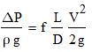
This Excel spreadsheet uses the Darcy-Weisbach equation to calculate liquid velocity in a pipe.  The Darcy-Weisbach equation describes the relationship between the pressure loss and liquid velocity in a pipe.

This is the equation employed in the spreadsheet.

• ΔP is the pressure loss in the pipe (Pa)
• ρ is the liquid density (kg m^-3)
• μ is the liquid viscosity (Pa s)
• g is the gravitational constant (9.81 m s^-2)
• L is the length of the pipe (m)
• D is the pipe diameter (m)
• V is the liquid velocity (m s^-1)
• f is the Darcy Fanning friction factor

For laminar flow (Re<2000), the friction factor f is 64/Re (where Re is the Reynolds Number). Ror turbulent flow the friction factor is given by the Haaland equation (although the Colebrook equation can be used instead).


The calculation is iterative, and requires the use of Excel's Goal Seek. However, this is automated in the spreadsheet so you only have to click a button and some VBA initiates Goal Seek for you.

The Darcy-Weisbach equation should only be used for steady-state incompressible flow. It can also be used for open-channel flows by replacing the diameter with the 4 R, where R is the hydraulic diameter.  The hydraulic diameter is simply the cross-sectional area divided by the wetted perimeter.

Download Excel Spreadsheet to use Darcy-Weisbach Equation to Calculate Liquid Velocity

Calculate Original Gas in Place with Excel

This Excel spreadsheet calculates the Original Gas in Place with a p/z plot.  Specifically, this spreadsheet fits the observed p/z data and cumulative gas product to the following curve

where

• (p/z) is the observed values of pressure over compressibility (collected during the life of a reservoir)
• Gp is corresponding cumulative gas production (again collected during the life of a reservoir)
• (p/z)_i is the initial value of pressure over compressibility of the system
• G is the original gas in place

This equation is simply a material balance, which many engineers use to determine the Original Gas in Place in volumetric natural gas reservoirs. It assumes a constant pore volume and includes the effect of gas expansion.  Note that the equation predicts a linear relationship between p/z and G

This screen grab illustrates the contents of the spreadsheet.

The spreadsheet is easy to follow.  It simply minimizes the sum-square residuals (difference between predicted and actual values of p/z) by varying G.  You can also choose to vary (p/z)_i in addition to G to minimize the sum-square residuals, but since this value is usually accurately measured, this is not recommended.

Fundamentally, this method is pretty simple to understand - we're simply locating the intercept on the x-axis (where p/z = 0) of a straight line fit of G against p/z, as illustrated by this picture.

This method of determining the Original Gas in Place is only suitable for normally pressurized gas reservoirs, where the gas expansion is the only significant factor contributing to gas production. This method, however, is not suitable for abnormally-pressurized reservoirs, where gas production is affected by formation compressibility (i.e.the expansion of sand, rock and water). Gas reservoirs are often abnormally-pressurized if they are in contact with aquifers

Download Excel spreadsheet to calculate Original Gas in Place

Model a Gas Orifice Meter with Excel

This Excel spreadsheet calculates the flowrate from the pressure drop across a gas orifice meter with the equations defined in ISO 5167.

Orifice meters use the pressure loss across a constriction (that is, the orifice plate) in a pipe to determine the flowrate.  While orifice meters are cost effective, they have several disadvantages. 

• The relationship between flowrate and pressure is non-linear,
• accurate values of the physical parameters are required,
• and high Reynolds numbers (>10⁴) are required for the greatest confidence in their accuracy, and the resulting pressure drop can be significant.

Accordingly, orifice meters are only used with the pressure drop is not critical, and accuracy is around 2% at best.

These are the equations implemented in the spreadsheet (as specified in ISO 5167)

Gas Orifice Meter Equations in ISO 5167

The notation is given below

• C is the discharge coefficient (only valid for the three standard tap positions given below)
• Re is the Reynolds number
• L₁ and L₂ are the upstream and downstream tap positions (m)
• P₁ and P₂ are the upstream and downstream pressures (Pa)
• D₁ and D₂ are the pipe and orifice diameters (m)
• V is the gas velocity in the pipe (m s^-1)
• ρ is the gas density (kg m^-3)
• μ is the gas viscosity (Pa s) 
• M is the molecular weight
• Y is the expansion coefficient
• Z is the gas compressibility factor
• K is the specific heat ratio
• R is the gas constant (8314 J kg^-1 k^-1)
• A_o is the cross-sectional area of the orifice (m²) 

There are three standard tap positions that determine the values of L₁ and L₂, as illustrated below. For corner taps, L₁ = L₂= 0, for D-D/2 taps L₁ = D₁ and L₂= D₁/2, and for flange taps L₁ = L₂= 1 inch. 

Tap positions in ISO 5167

The equations use the ideal gas law to calculate the gas density (you could override this with your own value), and are only valid for pipes with internal diameters from 50 mm to 1000 mm, and for pressure ratios greater than 0.75.

This is a screen grab of part of the spreadsheet.

The calculation is iterative: you need Re to calculate C, you need V to calculate Re, but you need C to calculate V.  Excel's Goal Seek functionality is used to iteratively solve the equations for the flowrate. This process is automated with a button - just fill in the parameters, click a button, and some VBA initiates Goal Seek with the correct settings

The spreadsheet provides an initial guess value for Re. This is used to calculate C and V. V is then used to calculate Re.  Excel's Goal Seek varies the guess value of Re until it matches the calculated value of Re.

By carefuly altering the equations (and the parameters used by Goal Seek), you could also solve for any other variable - for example, you could find the pressure drop for a specific flowrate (let me know if you need help in implementing this).

You'll find a spreadsheet  that models a liquid orifice meter here.

Visit http://excelcalculations.blogspot.com regularly for more free engineering spreadsheets.

Download Excel Spreadsheet to Calculate Flowrate in a Gas Orifice Meter (ISO 5167)

Multicomponent Equilibrium Flash Calculation

When a multicomponent liquid stream undergoes a sudden decrease in pressure (by, for example, flowing through a valve), part of the feed vaporizes.  The vapor product is richer in the more volatile components (i.e. those with a higher equilibrium constant) than the liquid product. This is known as an equilibrium flash, and is the basis of many unit operations in the process industries, including distillation.

This Excel spreadsheet implements an isothermal multicomponent equilibrium flash calculation. The spreadsheet includes a set of chemical components as the input feed (i.e. the molar amount in the feed stream, together with their K-values), but these can be easily modified.

We then use the Rachford-Rice equation to calculate the fraction of each component in the product streams. The equation is

where z_i is the mole fraction of component i in the liquid feed, K_i is the equilibrium constant (at the appropriate temperature and pressure) and β is the fraction of feed that is vaporised. Obviously, β is between 0 and 1.

We then solve the Rachford-Rice equation iteratively. All you need to do is find the value of β that makes the Rachford-Rice equation equal to zero using Excel's Solver function.  See the screengrab below for specific instructions.

The principles demonstrated in the spreadsheet are the basis of many other calculations that involve vapor-liquid equilibria, and are used in petroleum refineries, chemical plants and natural gas plants,

Download Excel spreadsheet for Multicomponent Equilibrium Flash

The Diet Problem

This Excel spreadsheet will help you find the cheapest combination of foods that fulfills a set of desired nutritional requirements.  This is known as The Diet Problem.  It's a classic example of linear programming and originates from the work of George Stigler, an economist who studied this problem in the 1940s. It was only in the 1950s with the development of the simplex algorithm by Dantzig that fast and accurate solutions became available.

Click this picture for an overview of the spreadsheet.

There are three primary steps in using this worksheet.

1. Specify the upper and lower bounds on your desired nutritional requirements.  You can set minimum and maximum values for the total calories, fat, saturated fat, trans fat, cholesterol, sodium, carbohydrates, fibre, sugar, protein, vitamin A, vitamin C, calcium and iron.
2. Specify a possible range of foods, their nutritional data and the cost per portion.  I've included a range of foods, but if you want to modify this list then http://www.nutritiondata.com has a database of foods and their nutritional qualities.
3. Use Excel's Solver to minimize the total cost (number of portions x cost per portion) while maintaining the nutritional requirements by varying the portions of each food (follow the steps in the picture above).

You may need to enable the Solver add-in via File>Options>Add-Ins.  I've saved my Solver model settings in the range A33:A57 in case you want to return to my defaults.

Of course, if you're seriously thinking about using this spreadsheet to optimize your diet, then I seriously suggest you reconsider - life is too short.

In fact, read George Dantzig's 1990 article The Diet Problem, in which he describes his attempt to follow a diet derived from this method.  He nearly overdosed on Bovril Bouillion cubes closely followed by two pounds of bran.  He ended up following his wife's advice and lost over 20 pounds. 

Download Excel spreadsheet to solve the Diet Problem

The Three Reservoir Problem

Introduction
This article discusses how you can solve the Three Reservoir Problem with Excel. First, we develop the governing equations by applying Bernoulli's Equation and the Continuity Equation. We then explore how these equations can be solved in Excel.

If you just want the tutorial spreadsheet, click here, but I encourage you to read the rest of the article so you understand how the spreadsheet was developed.  Read on for the Three Reservoir Problem solution.

Theory

Three reservoirs at different elevations are connected by a pipe network.  The common junction of the piping network is subject to an external demand Qj of 0.01 m3/s.  We will develop the theory required to calculate the flowrates in each pipe (Q1, Q2 and Q3), the head at the junction (Hj) and determine whether liquid is flowing into or out of each reservoir

Assuming that the liquid level in each reservoir is constant and the surface is open to atmosphere, the Bernoulli Equation for Reservoir i (where i=1, 2 and 3) is

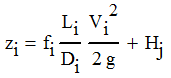
Equation 1

where zi is the elevation, fi is the friction factor, Li and Di are the length and diameter of the pipe connecting the reservoir to the junction, Vi is the liquid velocity and g is the gravitational constant.

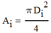
But the volumetric flowrate Qi and the cross sectional area Ai of the pipe are

Equation 2

Equation 3

Substituting Equations 2 and 3 into Equation 1 to eliminate Vi gives

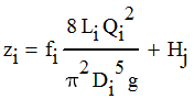
Equation 4

To determine whether liquid is flowing into or out of a reservoir, we need to preserve the sign on the Qi^2 term by writing Equation 4 thus

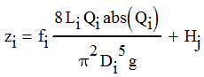
Equation 5

If Qi is positive, liquid is flowing out of the reservoir, and if Qi is negative, liquid is flowing into the reservoir.

We only need a few more relationships to completely specify the system.  The friction factor fi is given by the Haaland approximation to the Colebrook-White Equation,

where Rei is the Reynolds Number,

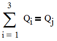
Additionally, the sum of the flowrates from each reservoir is equal to the external demand

Excel Implementation
Moving all terms in Equation 5 to the right-hand side gives

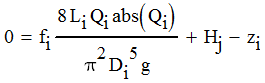
Equation 6

However, if we don't know the exact values of the flowrates in each pipeline (Qi) or the head at the junction (Hj) then we can define an error for each pipe.

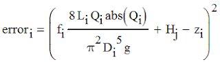
Equation 7

We'll use Excel's Solver add-in to find the values of Q1, Q2, Q3 and Hj that minimize the total error...

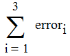
Equation 8

...while keeping the total flowrate at the junction equal to the external demand.

Equation 9

Step1. Specify fixed parameters (such as densities, viscosities, reservoir heights, pipe diameters and roughnesses etc)

Step 2. Set initial guess values for the flowrates in each pipe

  

Step 3. Specify calculated values

Step 4. Specify an initial guess value for the head at the junction, and the sum of all flowrates in each pipe (as given by Equation 9).  The External Demand will act as the constraint for Excel's Solver

Step 5.  Specify the errors for each pipeline (as given by Equation 7), and the total error (as given by Equation 8). 

We can now use Excel's Solver Add-in to find the flowrates (Q1, Q2 and Q3) and head at the junction (Hj) that minimize the total error (as set in Step 5) subject to the flowrate constraint (as set in Step 4).

Step 6.  Initiate Excel's Solver menu (if you haven't already, you'll need to load it in the File > Options > Add-ins menu)

Step 7. Make the appropriate changes in the Solver window such that you minimise the total error by varying the flowrates and the junction head while maintaining the external demand at a set value (for this example, I've set the external demand to 0.01 m3/s).  Additionally, set the solving method to GRG Nonlinear.

Step 8.  Click Solve.  After dismissing the following window, you'll find that the flowrates in each pipeline, and the junction head have changed.  Bear in mind that positive flowrates indicate flow out of a reservoir, while negative flowrates indicate liquid flow into a reservoir.

Step 9. We're not finished yet! Check that the Total Error specified in Step 5 is a very small number, and the External Demand (in Step 5) is equal to the value specified in Step 7.

Download Excel spreadsheet to solve The Three Reservoir Problem