Natural Gas Viscosity with Carr, Kobayashi, and Burrows Correlation

This Excel spreadsheet uses the Carr, Kobayashi, and Burrows correlation to calculate the viscosity of natural gas. The correlation is valid for sweet and sour gas.

The Carr, Kobayashi, and Burrows correlation was published in 1954. It is valid between temperatures of 32 F to 400 F, reduced pressures below 20, and CO₂, N₂ and H₂S concentrations below 15%.

The correlation was originally presented in graphs. However, this spreadsheet contains polynomial curve fits to the original graphs given by Dempsey (1965).

This spreadsheet also corrects calculates the viscosity (Standing & Katz, 1977) and pseudo-critical temperature/pressure of natural gas, but corrects for the presence of CO₂, N₂ and H₂S.

A spreadsheet to calculate the viscosity of natural gas based on the Lee, Gonzalez and Eakin correlation is also available; this method, however, is only valid for sweet natural gas.

Download Excel Spreadsheet to Calculate Natural Gas Viscosity using Carr, Kobayashi and Burrows

Calculate Original Gas in Place with Excel

This Excel spreadsheet calculates the Original Gas in Place with a p/z plot.  Specifically, this spreadsheet fits the observed p/z data and cumulative gas product to the following curve

where

• (p/z) is the observed values of pressure over compressibility (collected during the life of a reservoir)
• Gp is corresponding cumulative gas production (again collected during the life of a reservoir)
• (p/z)_i is the initial value of pressure over compressibility of the system
• G is the original gas in place

This equation is simply a material balance, which many engineers use to determine the Original Gas in Place in volumetric natural gas reservoirs. It assumes a constant pore volume and includes the effect of gas expansion.  Note that the equation predicts a linear relationship between p/z and G

This screen grab illustrates the contents of the spreadsheet.

The spreadsheet is easy to follow.  It simply minimizes the sum-square residuals (difference between predicted and actual values of p/z) by varying G.  You can also choose to vary (p/z)_i in addition to G to minimize the sum-square residuals, but since this value is usually accurately measured, this is not recommended.

Fundamentally, this method is pretty simple to understand - we're simply locating the intercept on the x-axis (where p/z = 0) of a straight line fit of G against p/z, as illustrated by this picture.

This method of determining the Original Gas in Place is only suitable for normally pressurized gas reservoirs, where the gas expansion is the only significant factor contributing to gas production. This method, however, is not suitable for abnormally-pressurized reservoirs, where gas production is affected by formation compressibility (i.e.the expansion of sand, rock and water). Gas reservoirs are often abnormally-pressurized if they are in contact with aquifers

Download Excel spreadsheet to calculate Original Gas in Place

Compressibility Factor Calculator for Excel

This Excel spreadsheet calculates the compressibility factor for natural gas using the Dranchuk-Abou-Kassem correlation.  Engineers need the compressibility factor to calculate natural gas flowrates (e.g., using the Weymouth Equation), viscosities (e.g. using the Lee, Gonzalez and Eakin correlation) or other properties

T_r is the reduced temperature, P_r is the reduced pressure, and ρ_r is the reduced density. The correlation is only valid for 0.20 ≤ P_r < 30, and 1.0 < T_r ≤ 30. The constants A1 to A11 were found by a best−fit to the Standing and Katz chart with an average absolute error of 0.585%.

The Dranchuk-Abou-Kassem equation is implicit; solving for Z requires an iterative solution method.  Several several methods exist in Excel, and the spreadsheet demonstrates two of these methods.

• A circular reference.  Make sure File>Options>Formulas>Enable iterative calculation is checked)
• Goal Seek.  Here we 
• guess a value for Z 
• use this to calculate ρ_r
• use ρ_r calculate Z
• use Goal Seek to minimize the difference between the guess and calculated values of Z by varying the guess value of Z

I've found that the result given via Goal Seek is more numerically stable (the circular reference often gives unrealistic results).  There's a button in the spreadsheet to initiate Goal Seek.

If you want Goal Seek to automatically recalculate the compressibility factor whenever the reduced temperature or pressure are changed, add this VBA to Sheet1 in the spreadsheet.

Private Sub Worksheet_Change(ByVal Target As Range)
Dim bSuccess As Boolean
    On Error Resume Next
    bSuccess = Range("diff").GoalSeek(0, Range("guessz"))
    On Error GoTo 0
    If Not bSuccess Then
        MsgBox "Goal Seek Failed for Compressibility Factor"
    End If
End Sub

You may also want to check out this Excel spreadsheet which uses the Beggs and Brill correlation to calculate the compressibility factor of natural gas.

Download Excel spreadsheet to calculate the compressibility factor with the Dranchuk-Abou-Kassem correlation

Calculate Viscosity of Natural Gas with Excel

This Excel spreadsheet will calculate the viscosity of natural gas. The spreadsheet uses the Lee, Gonzalez and Eakin correlation for the viscosity, and the CNGA (California Natural Gas Association) correlation for the compressibility factor.

The Lee, Gonzalez and Eakin correlation, only requires the pressure, temperature and molecular weight of the natural gas, and is relatively accurate compared to more complex methods of predicting viscosity.  It still widely used and accepted.

The CNGA compressibility factor correlation is suitable for pressures above 100 psig (below 100 psig, the compressibility factor is 1)

The Lee, Gonzalez and Eakin correlation was published in 1964 and accurately predicts the viscosity of natural gases with low non-hydrocarbon content, and for temperature between 100 F - 340 F, and pressures between 14.7-8000 psia. Additionally, the correlation is only suitable for sweet gases, and does not accurately describe sour gases (as described in this paper). The correlation has standard deviation of 2.7%, with a maximum deviation of 8.99%. The correlation is

Gas density is predicted by this correlation.

where ρ is the density in g/cm³, P is the pressure in psig, MW is the molecular weight (lb/lbmol), R is the gas constant (10.731 ft³ psi °R⁻¹ lb-mol⁻¹), T is the absolute temperature (°R) and Z is the compressibility factor.

Download Excel Spreadsheet to Calculate the Viscosity of Natural Gas

Calculate Water Content of Natural Gas with Excel

This Excel spreadsheet calculates the equilibrium water content of natural gas.  It uses a correlation derived from the McKetta-Wehe chart.  Originally published in 1958, the McKetta-Wehe chart is widely accepted in the natural gas industry.

There are several restrictions inherent to the McKetta-Wehe chart.

• This chart is suitable for sweet natural gas with a mole fraction of methane of more than 70%, and a relatively small fraction of heavy hydrocarbons. 
• Water content is overestimated at pressures of 70 bar absolute and over.
• The correlation is not suitable for natural gas in equilibrium with gas hydrates. The water content of these is a complex function of their composition and time.  Thus few reliable correlations exist, and thermodynamic models are usually used.
• The McKetta-Wehe chart should only be used at temperatures below which hydrate would form.

Download Excel Spreadsheet to Calculate the Water Content of Natural Gas

Compressibility Factor for Natural Gas

This Excel spreadsheet calculates the compressibility factor of natural gas using the Brill and Beggs correlation. Just enter the pressure, temperature, specific gravity and the mole fractions of N₂, CO₂ and H₂S.

The calculated value of the compressibility factor can be used to size natural gas pipelines (see my previous posts about the Weymouth, Panhandle A & B, IGT Distribution and Spitzglass spreadsheets for the sizing of natural gas pipelines).

The Beggs and Brill correlation was designed to calculate the compressibility of multiphase flow lines, and is essentially a best-fit equation to the standard Standing and Katz Z-factor chart. These are the equations as implemented in the Excel spreadsheet.

P_r and T_r are the critical temperatures and pressures and are calcualted from the mole fractions of N₂, CO₂ and H₂S specified in the spreadsheet. The correlation can't be used if the reduced temperature is below 0.92.

The compressibility factor models non-ideality in real gasses and is important when sizing long-distance natural gas pipelines.

Download Excel spreadsheet to calculate the Compressibility Factor.

The Spitzglass Equation for Sizing Gas Pipelines

Originally published in 1912, the Spitzglass Equation is used for sizing fuel gas pipes (although now it is superseded by better correlations).  Two versions of the equation exist;  one for low pressures (below 1 psi or 6.9 kPa) and another for medium pressures (above 1 psi or 6.9 kPa). However, both equations are typically used at near-atmospheric conditions, with pipe diameters below 10 inches (otherwise the friction factor is not accurately modeled).

This Excel spreadsheet solves both versions of the Spitzglass equations, with full units support.

The equations implemented are as follows

Spitzglass Low Pressure (<1 psi)

Spitzglass Medium Pressure (>1 psi)

The notation is given here.  These equations differ slightly to those versions typically presented in the literature because they include the effect of gas compressibility, and vertical pipe travel (i.e. potential energy).

I've also implemented other equations for sizing gas pipelines, including the Weymouth Equation, Panhandle Equation and the IGT Distribution Equation.

Download Excel spreadsheet to solve the Spitzglass Equation

The IGT Distribution Equation for Natural Gas Flow

I've previously blogged on the Weymouth and Panhandle A & B equations to predict the flow of natural gas through pipelines. Today, I'll complete this series of posts by presenting an Excel spreadsheet that calculates the IGT Equation (also known as the IGT Distribution Equation) for the flow of natural gas. The equation is particularly suitable for high pressure, high flowrates through steel or plastic/polyethylene pipes.

This is the IGT Equation as implemented in the spreadsheet (notation is defined here)

The spreadsheet allows you to choose between several units, and takes care of all unit conversions behind the scenes. It also enables you to model the effect of elevation changes on flowrates.

Download Excel spreadsheet for the IGT Distribution Equation

The Panhandle A and B Equations for Natural Gas Flow

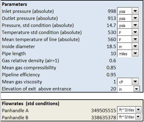
This Excel spreadsheet calculates the Panhandle A and B equations for the flow of natural gas through high pressure pipelines. You can choose between USCS (field units) or SI units, and even mix both (the spreadsheet does the unit conversion for you).

With Excel's Goal Seek function, you can also back-solve. For example, you can ask Excel to calculate the exit pressure that gives you a desired flowrate.

Weymouth (1912) developed the general gas flow equation. However, a limitation is that the friction factor can only be obtained iteratively. Hence simpler relationships based on the gas flow equation were developed, including the Weymouth equation and the Panhandle A (developed in the 1940s) and B (developed in 1956) equations.  These correlations simply substituted equations for the transmission factor (i.e. the friction factor) into the general gas flow equation.

The Panhandle equations are considered fairly accurate for Reynolds numbers between 4 million and 40 million.  Panhandle A is best suited for 12-60 inch diameter pipelines at pressures between 800 psia to 1500 psia. Panhandle B is most often used for pipes with a diameter of 36 inches or larger, and pressures above 1000 psia. Gas flows in pipelines with diameters of 15 inches or below are better modeled by the Weymouth equation.

As a caveat, the equations were originally developed for long pipelines; hence their use in shorter runs may not be appropriate

These are the equations implemented in the spreadsheet.

The notation is defined in a prior blog post that explores the Weymouth equation.

Download Excel spreadsheet for the Panhandle A and B equations for natural gas flow

The Weymouth Equation for High Pressure Gas Flow

This Excel spreadsheet helps you calculate pressures and flowrates using the the Weymouth Equation, a relationship usually used in long-distance natural gas pipelines.

The Weymouth Equation gives more conservative results than the Panhandle equations, and is hence more frequently used.  It is valid for steady-state adiabatic (isothermal) flow.  The version of the Weymouth equation used in this spreadsheet also accounts for elevation differences between the pipe entrance and exit.

In Imperial units, the Weymouth equation is

• Tsc and Psc are the temperature and pressure at standard conditions, in absolute Fahrenheit
• Tm is the average temperature of the gas line, in absolute Fahrenheit
• P1 and P2 are the pressures at the pipe entrance and exit, in absolute psi
• L is the length of the pipe, in miles
• G is the relative gas density with respect to air
• Z is the gas compressibility
• E is the pipeline efficiency
• Le is the effective length of the pipeline
• Δz is the elevation of the pipe exit with respect to the entrance in feet
• Q is the flowrate, in standard cubic feet per day

The gas compressibility Z and density are calculated at an average pressure and temperature, defined below.

The equations given above use several empirical factors, and normally the input parameters would need to be specified in specific units.  However, I've programmed the spreadsheet to handle the unit conversions for you.  You simply specify the input units using drop-down menus.

For dry gas fields, the pipeline efficiency is generally around 0.92, casing-head gas would have a pieline efficiency of 0.77, while gas and condensate pipes have an efficiency of 0.66

Download Weymouth Equation Calculator for Excel